This web app is a simple MNIST classifier with an explanation component. The black square below is a canvas you can draw on (with a finger or a mouse,
depending on your device). After clicking submit, the canvas content is sent to the model for classification. The results show the model's softmax output
(the probabilities that the input belongs to each class), followed by an explanation of why the model thinks the highest-probability class is the correct
one. An explanation of the explanation process is in the paragraph below. The interesting part of the explanation is that we can figure out how to fool a
model into confidently returning a response even if we just give it something semantically meaningless (see examples below). This all shows us just how
easy it is to fool AI, and maybe why we shouldn't put too much trust in its results.
Explanation
This classifier returns three pieces of data. The original input image, the softmax probabilities of the classifier, and the explanation
for why a classification has been made. The explanation is the most interesting part because we can have the model explain the classification
it has given, which opens up the otherwise closed-box AI system.
The heat map shows us the parts of the image that are important to the classification. Red indicates a positive contribution to the class, grey
does not contribute to the class, and blue areas reduce the class probability. This is produced using Integrated Gradients
from the Captum library.
To compute the integrated gradients of a model \(F\), we start with the input to the model \(x\) and a baseline \(x'\). The baseline is essentially an input
that should elicit no meaningful response from the network (a response that is as uniform as possible). In the case of images, this would be a black image.
We select a dimension \(i\) (a pixel in the case of images) and take a path integral of the gradient along a linear interpolation from \(x\) to \(x'\):
\[
IG_i(x) := (x_i - x_i') \cdot \int^1_{\alpha=0} \frac{\partial F (x' + \alpha (x-x'))}{\partial x_i} d\alpha
\]
Since \(\alpha \in [0,1]\), we gradually move along the path from a completely black image to the original colour version. While this is happening,
we're paying close attention to the rate of change of the model output with respect to \(x_i\). This allows us to understand the importance of dimension \(i\) to
the classification. Doing this for each pixel (or group of pixels) will enable us to see what parts of the input contribute most strongly to the output!
Let's Fool AI
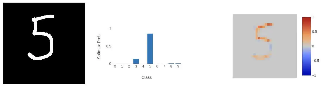
We can start with a basic classification task.
From this we can see that the top of the 5 is important (a squared off 'c'), followed by the end of the hook. So what happens if we remove the centre part of the 5?
It's still pretty confident it's a 5. But as a human we can kind of tell it's still a 5. But from that last run we can see that we can represent a 5 with just three lines:
The model is still quite sure that's a 5!
⚠️ If the canvas is green the page is still loading, please wait until it turns black before starting to draw!
 From this we can see that the top of the 5 is important (a squared off 'c'), followed by the end of the hook. So what happens if we remove the centre part of the 5?
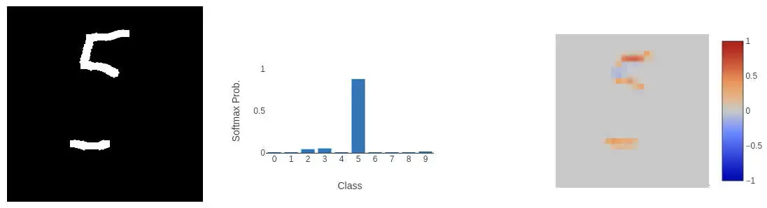 It's still pretty confident it's a 5. But as a human we can kind of tell it's still a 5. But from that last run we can see that we can represent a 5 with just three lines:
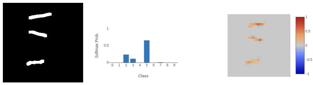 The model is still quite sure that's a 5!